Usage examples
Materials
In this protocol we show how to analyze genomic variants using the SnpEff pipeline.
Computer hardware: The materials required for this protocol are:
- a computer running a Unix operating system (Linux, OS.X),
- at least 16GB of RAM
- at least 8Gb of free disk space,
- Java
- a reasonably fast internet connection
Users of Windows computers can install CygWin, a free Linux-like environment for Windows, although the precise commands listed in the protocol may need to adapted.
Software: We use the SnpEff annotation program and its companion tool SnpSift. These programs can perform annotation, primary impact assessment and variants filtering, as well as many other tasks beyond the scope of this protocol. We highly recommend reading their comprehensive documentation available here.
Before starting the protocol, it is necessary to download and install SnpEff. To do this, open a Unix, Linux or Cygwin shell and execute the following commands:
# Move to home directory
cd

# Download and install SnpEff
curl -v -L 'https://snpeff-public.s3.amazonaws.com/versions/snpEff_latest_core.zip' > snpEff_latest_core.zip
unzip snpEff_latest_core.zip
Notes:
- SnpEff & SnpSift annotation software used in this protocol are under very active development and some command line option may change in the future.
- The standard installation is to add the package in the "$HOME/snpEff" directory (where $HOME is your home directory). To install SnpEff elsewhere, update the "data.dir" parameter in your "snpEff.config" file, as described in the SnpEff documentation.
Once SnpEff is installed, we will enter the following commands to download the pre-built human database (GRCh37.75) that will be used to annotate our data.
cd snpEff
java -jar snpEff.jar download -v GRCh37.75
A list of pre-built databases for all other species is available by running the following command:
java -jar snpEff.jar databases
Example 1: Coding variants
We show how to use SnpEff & SnpSift to annotate, prioritize and filter coding variants.
Dataset: In this genomic annotation example, we use a simulated dataset to show how to find genetic variants of a Mendelian recessive disease, Cystic fibrosis, caused by a high impact coding variant, a nonsense mutation in CFTR gene (G542*).
The data files come from the publicly available "CEPH_1463" dataset, sequenced by Complete Genomics, and contains sequencing information for a family consisting of 4 grandparents, 2 parents and 11 siblings.
Although these are healthy individuals, we artificially introduced a known Cystic fibrosis mutation on three siblings (cases) in a manner that was consistent with the underlying haplotype structure.
We now download and un-compress the example data used in this protocol, which, for reasons of space and time, is limited to only chromosome 7 and 17:
# Go to SnpEff's dir
cd ~/snpEff

# Download sample data
curl -v -L 'https://datasetsnpeff-public.s3.amazonaws.com/dataset/protocols.zip?sv=2019-10-10&st=2020-09-01T00%3A00%3A00Z&se=2050-09-01T00%3A00%3A00Z&si=prod&sr=c&sig=isafOa9tGnYBAvsXFUMDGMTbsG2z%2FShaihzp7JE5dHw%3D' > protocols.zip
unzip protocols.zip
The goal in this example is to use SnpEff to find a mutation causing a Mendelian recessive trait. This will be done using a dataset of variant calls for chromosome 7 from a pedigree of 17 healthy individuals, sequenced by Complete Genomics, in which a coding variant causing cystic fibrosis was artificially introduced in three siblings (see Materials). For the purpose of this example, we assume that we do not know the causative variant, but that we know that we are dealing with a Mendelian recessive disorder, where the three siblings are affected (cases), but the 14 parents and grandparents are not (controls).
Genomic variants are usually provided in a VCF file containing variant information of all the samples; storing the variant data in a single VCF file is the standard practice, not only because variant calling algorithms have better accuracy when run on all samples simultaneously, but also because it is much easier to annotate, manipulate and compare individuals when the data is stored and transferred together. A caveat of this approach is that VCF files can become very large when performing experiments with thousands of samples (from several Gigabytes to Terabytes in size).
In the following protocol, SnpEff will add annotation fields to each variant record in the input VCF file. We will then use SnpSift, a filtering program to extract the most significant variants having annotations meeting certain criteria.
Step 1: Primary variant annotation and quality control.
Our first step is to annotate each of the ~500,000 variants contained in the VCF file. By default, SnpEff adds primary annotations and basic impact assessment for coding and non-coding variants as described above. SnpEff has several command line options that can be used in this annotation stage and which are described in detail in the online manual.
In this example, we annotate (all these annotations are activated by default when using SnpEff):
- loss of function and nonsense mediated decay predictions;
- protein domain annotations from the curated NextProt database;
- putative transcription factor binding sites from the ENSEMBL 'Regulatory Build' and Jaspar database;
- use HGVS notation for amino acid changes; and
- to create a web page summarizing the annotation results in "ex1.html" (option
-stats):java -Xmx8g -jar snpEff.jar -v -stats ex1.html GRCh37.75 protocols/ex1.vcf > protocols/ex1.ann.vcf
SnpEff produces three output files :
- the HTML file containing summary statistics about the variants and their annotations;
- an annotated VCF file; and
- a text file summarizing the number of variant types per gene.
Creation of the summary files can be de-activated to speed up the program (for example, when the application is used together with Galaxy). By default, the statistics file "ex1.html" is a standard HTML file that can be opened in any web browser to view quality control (QC) metrics. It can also be created in comma-separated values format (CSV) to be used by downstream processing programs as part of an automated pipeline. In our example, the summary file contains basic quality control statistics calculated from the variant file: for our data, the Ts/Ts ratio is close to 2.0 (Figure 1c) and missense / silent ratio is around 1.0 (Figure 1d), both of which are expected for human data (but these numbers may differ for other species).
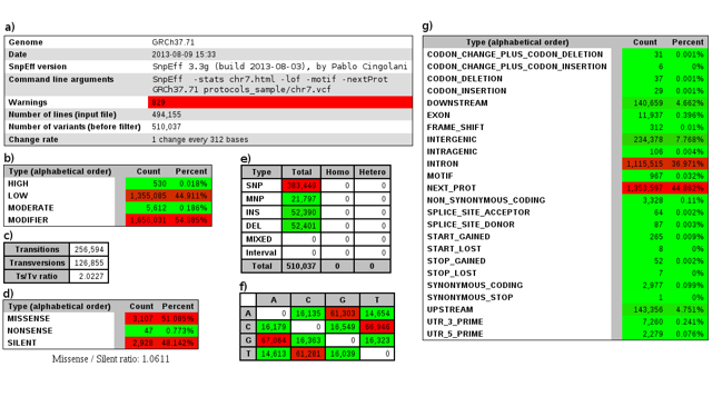
Large deviations from the expected values for the organism being sequenced might indicate problems with either the sequencing or variant calling pipelines. The summary file also contains QC information for the gene annotation used as input. In this example, 829 warnings (Figure 1a) were identified as a result of possible genomic annotation errors or small inconsistencies identified in the reference genome so we have to be careful analyzing those genes/transcripts. Other summary statistics are available, such as variant types (Figure 1e), variants effects (Figure 1d and 1g), and primary impacts (Figure 1b and 1g).
Step 2: Counting variants in case and control subjects.
In the first step of our protocol, SnpEff created a VCF file with half million annotated variants. Rather than scanning each annotation manually, we will use the SnpSift program to create a filter that will identify a small subset of variants with interesting functional properties. Since the VCF files used in most sequencing studies are even larger than the one in this example, our overall approach is to start by creating a filter using a very restrictive set of criteria. If no relevant variant is found using this stringent filter, we will relax the criteria to include variants with lower predicted impact.
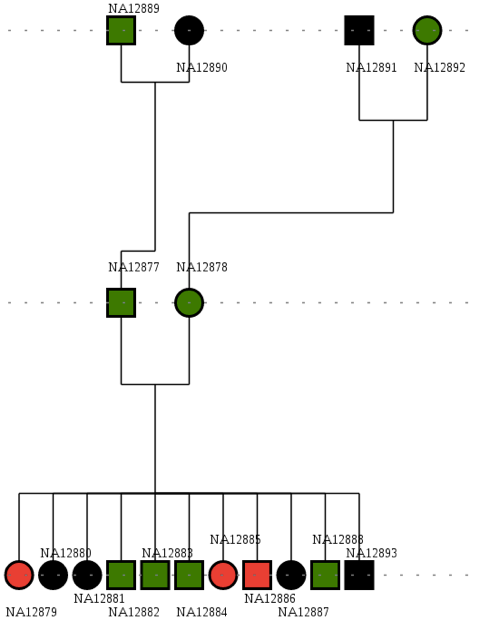
In our example, since the pedigree is consistent with a Mendelian recessive disease, so we will first use SnpEff to find high impact variants that are homozygous in cases and either absent or heterozygous in controls. This provides a very strong genetic argument to select the promising variants and will be used as the first step in our filter. To do this, we will identify the case and control samples by providing SnpEff with pedigree information using a "TFAM" file (a standard file format used to describe pedigrees). In our example, the TFAM file ("pedigree.tfam") identifies the three cases (NA12879, NA12885, NA12886), and lists the other family members as controls. The "caseControl" command instructs the SnpSift program to count the number homozygous non-reference, heterozygous and allele count (number of non-reference alleles in each DNA sample) for both cases and controls groups (running time: ~60 minutes):
java -Xmx1g -jar SnpSift.jar \
    caseControl \
    -v \
    -tfam protocols/pedigree.tfam \
    protocols/ex1.ann.vcf \
    > protocols/ex1.ann.cc.vcf
This analysis creates an output VCF file ("ex1.ann.cc.vcf") by adding new information to the INFO field for each variant: this includes information such as Cases=1,1,3 and Controls=8,6,22 which correspond to the number of homozygous non-reference, heterozygous and total allele counts in cases and controls for each variant.
The program also calculates basic statistics for each variant based on the allele frequencies in the two groups using different models, which can be useful as a starting point for more in-depth statistical analysis.
Step 3: Filtering variants.
We can use the SnpSift filter command to reduce the number of candidate loci base on alleles in cases and controls.
SnpSift filter allows users to create powerful filters that select variants using Boolean expressions containing data from the VCF fields.
The expression we use to filter the VCF file "ex1.ann.vcf" is developed as follows.
We expect all the three cases and none of the controls to be homozygous for the mutation.
This is expressed using the following filter: (Cases[0] = 3) & (Controls[0] = 0)
The full command line is:
cat protocols/ex1.ann.cc.vcf | java -jar SnpSift.jar filter \
    "(Cases[0] = 3) & (Controls[0] = 0)" \
    > protocols/ex1.filtered.hom.vcf
The filtered output file, filtered.hom_cases.vcf, contains over 400 variants satisfying our criteria.
This is still too large to analyze by hand, so can we can add another filter to see if any of these variants is expected to have a high impact.
To identify variants where any of these impacts is classified as either HIGH or MODERATE we add the condition (ANN[*].IMPACT = 'HIGH') | (ANN[*].IMPACT = 'MODERATE').
The new filtering commands become:
cat protocols/ex1.ann.cc.vcf \
    | java -jar SnpSift.jar filter \
    "(Cases[0] = 3) & (Controls[0] = 0) & ((ANN[*].IMPACT = 'HIGH') | (ANN[*].IMPACT = 'MODERATE'))" \
    > protocols/ex1.filtered.vcf
stop_gained loss of function variant, whereas the other one is a missense_variant amino acid change.
The first one is a known Cystic fibrosis variant.
$ cat protocols/ex1.filtered.vcf     | ./scripts/vcfInfoOnePerLine.pl
7   117227832   .   G    T      .    .
                                AC      14
                                AN      22
                                ANN     T|stop_gained|HIGH|CFTR|ENSG00000001626|transcript|ENST00000003084|protein_coding|12/27|c.1624G>T|p.Gly542*|1756/6128|1624/4443|542/1480||
                                ANN     T|stop_gained|HIGH|CFTR|ENSG00000001626|transcript|ENST00000454343|protein_coding|11/26|c.1441G>T|p.Gly481*|1573/5949|1441/4260|481/1419||
                                ANN     T|stop_gained|HIGH|CFTR|ENSG00000001626|transcript|ENST00000426809|protein_coding|11/26|c.1534G>T|p.Gly512*|1534/4316|1534/4316|512/1437||WARNING_TRANSCRIPT_INCOMPLETE
                                ANN     T|sequence_feature|LOW|CFTR|ENSG00000001626|topological_domain:Cytoplasmic|ENST00000003084|protein_coding||c.1624G>T||||||
                                ANN     T|sequence_feature|LOW|CFTR|ENSG00000001626|domain:ABC_transporter_1|ENST00000003084|protein_coding||c.1624G>T||||||
                                ANN     T|sequence_feature|LOW|CFTR|ENSG00000001626|beta_strand|ENST00000003084|protein_coding|12/27|c.1624G>T||||||
                                ANN     T|sequence_feature|LOW|CFTR|ENSG00000001626|beta_strand|ENST00000454343|protein_coding|11/26|c.1441G>T||||||
                                ANN     T|upstream_gene_variant|MODIFIER|AC000111.5|ENSG00000234001|transcript|ENST00000448200|processed_pseudogene||n.-1C>A|||||1362|
                                ANN     T|downstream_gene_variant|MODIFIER|CFTR|ENSG00000001626|transcript|ENST00000472848|processed_transcript||n.*148G>T|||||29|
                                LOF     (CFTR|ENSG00000001626|11|0.27)
                                NMD     (CFTR|ENSG00000001626|11|0.27)
                                Cases   3
                                Cases   0
                                Cases   6
                                Controls        0
                                Controls        8
                                Controls        8
                                CC_TREND        9.111e-04
                                CC_GENO NaN
                                CC_ALL  4.025e-02
                                CC_DOM  6.061e-03
                                CC_REC  1.000e+00

17    39135205   .    ACA       GCA,GCG .       .
                                AC      16
                                AC      8
                                AN      31
                                ANN     GCG|missense_variant|MODERATE|KRT40|ENSG00000204889|transcript|ENST00000377755|protein_coding||c.1045_1047delTGTinsCGC|p.Cys349Arg|1082/1812|1045/1296|349/431||
                                ANN     GCG|missense_variant|MODERATE|KRT40|ENSG00000204889|transcript|ENST00000398486|protein_coding||c.1045_1047delTGTinsCGC|p.Cys349Arg|1208/1772|1045/1296|349/431||
                                ANN     GCA|synonymous_variant|LOW|KRT40|ENSG00000204889|transcript|ENST00000377755|protein_coding|6/7|c.1047T>C|p.Cys349Cys|1082/1812|1047/1296|349/431||
                                ANN     GCA|synonymous_variant|LOW|KRT40|ENSG00000204889|transcript|ENST00000398486|protein_coding|8/9|c.1047T>C|p.Cys349Cys|1208/1772|1047/1296|349/431||
                                ANN     GCA|sequence_feature|LOW|KRT40|ENSG00000204889|region_of_interest:Coil_2|ENST00000398486|protein_coding|6/9|c.1047T>C||||||
                                ANN     GCG|sequence_feature|LOW|KRT40|ENSG00000204889|region_of_interest:Coil_2|ENST00000398486|protein_coding|7/9|c.1045_1047delTGTinsCGC||||||
                                ANN     GCA|sequence_feature|LOW|KRT40|ENSG00000204889|region_of_interest:Rod|ENST00000398486|protein_coding|3/9|c.1047T>C||||||
                                ANN     GCG|sequence_feature|LOW|KRT40|ENSG00000204889|region_of_interest:Rod|ENST00000398486|protein_coding|3/9|c.1045_1047delTGTinsCGC||||||
                                ANN     GCA|3_prime_UTR_variant|MODIFIER|KRT40|ENSG00000204889|transcript|ENST00000461923|nonsense_mediated_decay|8/9|n.*509T>C|||||2348|
                                ANN     GCG|3_prime_UTR_variant|MODIFIER|KRT40|ENSG00000204889|transcript|ENST00000461923|nonsense_mediated_decay|8/9|n.*507_*509delTGTinsCGC|||||2346|
                                ANN     GCA|downstream_gene_variant|MODIFIER|AC004231.2|ENSG00000234477|transcript|ENST00000418393|antisense||n.*815A>G|||||3027|
                                ANN     GCG|downstream_gene_variant|MODIFIER|AC004231.2|ENSG00000234477|transcript|ENST00000418393|antisense||n.*815_*815delACAinsGCG|||||3027|
                                ANN     GCA|non_coding_exon_variant|MODIFIER|KRT40|ENSG00000204889|transcript|ENST00000461923|nonsense_mediated_decay|8/9|n.*509T>C||||||
                                ANN     GCG|non_coding_exon_variant|MODIFIER|KRT40|ENSG00000204889|transcript|ENST00000461923|nonsense_mediated_decay|8/9|n.*507_*509delTGTinsCGC||||||
                                Cases   3
                                Cases   0
                                Cases   6
                                Controls        0
                                Controls        12
                                Controls        18
                                CC_TREND        7.008e-02
                                CC_GENO NaN
                                CC_ALL  1.700e-01
                                CC_DOM  1.231e-01
                                CC_REC  1.000e+00
java -jar SnpSift.jar pedShow \
    protocols/pedigree.tfam \
    protocols/ex1.filtered.vcf \
    protocols/chart
Step 4. Using clinical databases.
So far, since the purpose of the example was to show how annotations and filtering are performed to uncover new variants, we assumed that the causative variant was not known. In reality the variant is known and databases, such as ClinVar, have this information in convenient VCF format that can be used for annotations.
We can annotate using ClinVar by using the following command:
java -Xmx1g -jar SnpSift.jar \
    annotate \
    -v \
    protocols/db/clinvar_00-latest.vcf \
    protocols/ex1.ann.cc.vcf \
    > protocols/ex1.ann.cc.clinvar.vcf
Our variant of interest is then annotated as "Cystic Fibrosis" (to find the variant, we filter for variants having ClinVar annotation "CLNDBN" that are in CFTR gene and have a stop_gained annotation):
$ cat protocols/ex1.ann.cc.clinvar.vcf \
    | java -jar SnpSift.jar filter \
    "(exists CLNDBN) & (ANN[*].EFFECT has 'stop_gained') & (ANN[*].GENE = 'CFTR')" \
    > protocols/ex1.ann.cc.clinvar.filtered.vcf

$ cat protocols/ex1.ann.cc.clinvar.filtered.vcf | ./scripts/vcfInfoOnePerLine.pl
7    117227832    rs113993959      G    T       .    .
                                                AC              14
                                                AN              22
                                                ANN             T|stop_gained|HIGH|CFTR|ENSG00000001626|transcript|ENST00000003084|protein_coding|12/27|c.1624G>T|p.Gly542*|1756/6128|1624/4443|542/1480||
                                                ANN             T|stop_gained|HIGH|CFTR|ENSG00000001626|transcript|ENST00000454343|protein_coding|11/26|c.1441G>T|p.Gly481*|1573/5949|1441/4260|481/1419||
                                                ANN             T|stop_gained|HIGH|CFTR|ENSG00000001626|transcript|ENST00000426809|protein_coding|11/26|c.1534G>T|p.Gly512*|1534/4316|1534/4316|512/1437||WARNING_TRANSCRIPT_INCOMPLETE
                                                ANN             T|sequence_feature|LOW|CFTR|ENSG00000001626|topological_domain:Cytoplasmic|ENST00000003084|protein_coding||c.1624G>T||||||
                                                ANN             T|sequence_feature|LOW|CFTR|ENSG00000001626|domain:ABC_transporter_1|ENST00000003084|protein_coding||c.1624G>T||||||
                                                ANN             T|sequence_feature|LOW|CFTR|ENSG00000001626|beta_strand|ENST00000003084|protein_coding||c.1624G>T||||||
                                                ANN             T|sequence_feature|LOW|CFTR|ENSG00000001626|beta_strand|ENST00000454343|protein_coding||c.1441G>T||||||
                                                ANN             T|upstream_gene_variant|MODIFIER|AC000111.5|ENSG00000234001|transcript|ENST00000448200|processed_pseudogene||n.-1C>A|||||1362|
                                                ANN             T|downstream_gene_variant|MODIFIER|CFTR|ENSG00000001626|transcript|ENST00000472848|processed_transcript||n.*148G>T|||||29|
                                                LOF             (CFTR|ENSG00000001626|11|0.27)
                                                NMD             (CFTR|ENSG00000001626|11|0.27)
                                                Cases           3
                                                Cases           0
                                                Cases           6
                                                Controls        0
                                                Controls        8
                                                Controls        8
                                                CC_TREND        9.111e-04
                                                CC_GENO         NaN
                                                CC_ALL          4.025e-02
                                                CC_DOM          6.061e-03
                                                CC_REC          1.000e+00
                                                ASP             true
                                                CLNACC          RCV000007535.6|RCV000058931.3|RCV000119041.1
                                                CLNALLE         1
                                                CLNDBN          Cystic_fibrosis|not_provided|Hereditary_pancreatitis
                                                CLNDSDB         GeneReviews:MedGen:OMIM:Orphanet:SNOMED_CT|MedGen|GeneReviews:MedGen:OMIM:Orphanet:SNOMED_CT
                                                CLNDSDBID       NBK1250:C0010674:219700:ORPHA586:190905008|CN221809|NBK84399:C0238339:167800:ORPHA676:68072000
                                                CLNHGVS         NC_000007.13:g.117227832G>T
                                                CLNORIGIN       1
                                                CLNREVSTAT      prof|single|single
                                                CLNSIG          5|5|5
                                                CLNSRC          CFTR2|HGMD|OMIM_Allelic_Variant|OMIM_Allelic_Variant
                                                CLNSRCID        G542X|CM900049|602421.0009|602421.0095
                                                GENEINFO        CFTR:1080
                                                LSD             true
                                                NSN             true
                                                OM              true
                                                PM              true
                                                PMC             true
                                                REF             true
                                                RS              113993959
                                                RSPOS           117227832
                                                S3D             true
                                                SAO             1
                                                SSR             0
                                                VC              SNV
                                                VLD             true
                                                VP              0x050268000605040002110100
                                                WGT             1
                                                dbSNPBuildID    132
Example 2: Software Integration (GATK & Galaxy)
Software Integration (Optional): Sequence analysis software is often run in high performance computers combining several programs into processing pipelines. Annotations and impact assessment software needs to provide integration points with other analysis steps of the pipeline.
In the following paragraphs we describe how to integrate SnpEff with two programs commonly used in sequencing analysis pipelines:
- Genome Analysis toolkit (GATK 2), a command-line driven software;
- Galaxy 3, a web based software.
GATK
The Genome Analysis Toolkit 2 is one of the most popular programs for bioinformatics pipelines.
Annotations can be easily integrated into GATK using SnpEff and GATK's VariantAnnotator module. Here we show how to annotate a file using SnpEff and GATK, as an alternative way of performing step 1. You should perform this step only if your processing pipeline is based on GATK: compared to running SnpEff from the command line, the results obtained when using GATK will only contain the highest impact annotation for each variant. This was a conscious trade-off made by the designers of GATK, partly because most biologists do this implicitly when reading a list of variants, but also to improve the readability and reduce the size of the annotation results.
The method requires two steps:
- Annotating a VCF file using SnpEff
- Using GATK's VariantAnnotator to incorporate those annotations into the final VCF file.
When using SnpEff for GATK compatibility, we must use the -o gatk command line option:
java -Xmx8g -jar snpEff.jar \
    -v \
    -o gatk \
    GRCh37.75 \
    protocols/ex1.vcf \
    > protocols/ex1.ann.gatk.vcf
Next, we process these variants using GATK. For this step to work correctly, we need to make sure that our data files are compatible with the requirements GATK places on reference genomes (see GATK's documentation for more details):
- in the fasta file, chromosomes are expected to be sorted in karyotypic order;
- a genome fasta-index file must be available; and
- a dictionary file must be pre-computed.
Assuming these requirements are satisfied, we can run the following command, which will produce a GATK annotated file ("ex1.gatk.vcf"):
java -Xmx8g -jar $HOME/tools/gatk/GenomeAnalysisTK.jar \
    -T VariantAnnotator \
    -R $HOME/genomes/GRCh37.75.fa \
    -A SnpEff \
    --variant protocols/ex1.vcf \
    --snpEffFile protocols/ex1.ann.gatk.vcf \
    -L protocols/ex1.vcf \
    -o protocols/ex1.gatk.vcf
Note: We assumed GATK is installed in "$HOME/tools/gatk/" and the reference genome is contained in "$HOME/genomes/GRCh37.75.fa" These file locations should be adapted to the actual path in your computer.
Galaxy
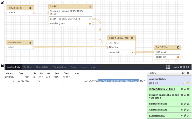
Anther popular tool in bioinformatics is Galaxy 3, which allows pipelines to be created in a web environment using graphical interface, making it flexible and straightforward to use. SnpEff provides Galaxy modules.
Once these modules are installed, we can run our sample annotation pipeline in Galaxy.
Example 3: Non-Coding variants
We show how to use SnpEff & SnpSift to annotate, prioritize and filter non-coding variants.
Dataset: This example shows how to perform basic annotation of non-coding variants. It is based on a short list of 20 non-coding that were identified by sequencing a 700 kb region surrounding the gene T-box transcription factor (TBX5) in 260 patients with congenital heart disease 67. TBX5 is a transcription factor that plays a well-established dosage-dependent role in heart and limb development. Coding mutations in TBX5 have been frequently identified in patients with Holt-Oram syndrome, which is associated with abnormal hand, forearm and cardiac development.
Data source: Regulatory variation in a TBX5 enhancer leads to isolated congenital heart disease.
Step 1. Annotating variants.
We will perform non-coding variant annotation using SnpEff following a similar approach to Procedure I. In this case, we construct a command line that instructs SnpEff to include motif information ("-motif") and putative transcription factor binding sites (TFBS) identified in the ENSEMBL Regulatory Build and the Jaspar database:
java -Xmx8g -jar snpEff.jar \
    -v \
    -motif \
    GRCh37.75 \
    protocols/ex2.vcf \
    > protocols/ex2.ann.basic.vcf
Step 2. Adding custom regulatory information.
A quick scan through the results shows that most variants are catalogued as "INTERGENIC", and none of them is associated with a known TFBS. This is not surprising since TFBS are small and also because regulatory elements involved in cardiac or limb development may not be widely active in commonly studied adult tissues. In this case, basic annotations did not provide additional information that can be used to narrow down the list of candidate SNVs.
To solve this, the authors examined data from other sources, including ChIP-seq data for H3K4me1 (a post-translationally modified histone protein found in transcriptionally active genome regions, including enhancers and promoters).
Data produced from ChIP-Seq analysis are frequently published in BED, BigBed or similar formats, which can be used directly by SnpEff by adding the -interval command line option.
This command line option can be used to add annotations using ChIP-Seq experiments from the ENCODE and Epigenome Roadmap projects: since multiple -interval options are allowed in each command line, it is a simple way to combine several annotations:
java -Xmx8g -jar snpEff.jar \
    -v \
    -motif \
    -interval protocols/ex2_regulatory.bed \
    GRCh37.75 \
    protocols/ex2.vcf \
    > protocols/ex2.ann.vcf
-interval command line option are annotated as "CUSTOM[ex2_regulatory]" : the name in brackets identifies the file name provided to distinguish multiple annotation files.
Step 3. Adding conservation information.
In order to refine our search, we can also look for variants in highly conserved non-coding bases. SnpEff natively supports PhastCons scores, but can also add annotations based on any other user-defined score provided as a Wig or VCF file.
The command line for annotating using the PhastCons score is:
java -Xmx1g -jar SnpSift.jar \
    phastCons \
    -v \
    protocols/phastcons \
    protocols/ex2.ann.vcf \
    > protocols/ex2.ann.cons.vcf
Now we can filter our results looking for a highly conserved SNP in the regulatory region. We do this by using a "SnpSift filter" command and the appropriate Boolean expression:
cat protocols/ex2.ann.cons.vcf \
    | java -jar SnpSift.jar filter \
    "(ANN[*].EFFECT = 'CUSTOM[ex2_regulatory]') & (exists PhastCons) & (PhastCons > 0.9)" \
    > protocols/ex2.filtered.vcf
SnpSift filter supports a flexible syntax to create Boolean expressions using the annotation data that provides a versatile way to prioritize shorter lists of SNPs for subsequent validation. This syntax is described in detail in the online manual. In this example, our filter results in only two candidate SNPs, one of which was extensively validated in the original study and is assumed to be causative.
The principles illustrated in our example for a small set of SNVs can be applied to millions of variants from whole genome sequencing experiments. Similarly, although we filtered the SNVs using "custom" ChIP-seq data that provided in the original study, regulatory information from public Encode or Epigenome Roadmap datasets could be used in a first line investigation before generating our own Chip-seq or RNA-seq data using disease-relevant cells and tissues.
Example 4: Sequencing data analysis
Here we show an example on how to get from Sequencing data to an annotated variants file.
Sequencing data example
Warning
This is an extremely simplified version on how to analyze the data from scratch. This is not meant to be a tutorial on sequencing analysis as it would be way beyond the scope of this handbook.
Let's assume you have sequence data in FASTQ format (file "s.fastq") and your reference genome is dm5.34 (fly genome)
# Download the genome, uncompress and rename file
wget ftp://ftp.flybase.net/genomes/Drosophila_melanogaster/dmel_r5.34_FB2011_02/fasta/dmel-all-chromosome-r5.34.fasta.gz
gunzip dmel-all-chromosome-r5.34.fasta.gz
mv dmel-all-chromosome-r5.34.fasta dm5.34.fasta

# Create a genome index (we assume you installed BWA)
bwa index -bwtsw dm5.34.fasta

# Map sequences to the genome: Create SAI file
bwa aln -bwtsw dm5.34.fasta s.fastq > s.sai

# Map sequences to the genome: Create SAM file
bwa samse dm5.34.fasta s.sai s.fastq > s.sam

# Create BAM file (we assume you installed SamTools)
samtools view -S -b s.sam > s.bam

# Sort BAM file (will create s_sort.bam)
samtools sort s.bam s_sort

# Create VCF file (BcfTools is part of samtools distribution)
samtools mpileup -uf dm5.34.fasta s_sort.bam | bcftools view -vcg - > s.vcf

# Analyze variants using snpEff
java -Xmx8g -jar snpEff.jar dm5.34 s.vcf > s.ann.vcf
This highly simplified sequencing data analysis pipeline, has these basic steps:
- Index the reference genome (bwa)
- Map reads to reference genome (bwa)
- Call variants (bcftools)
- Annotate variants (SnpEff)
Example 5: Filter out variants (dbSnp)
Here we show an example on how to get from Sequencing data to an annotated variants file.
These are slightly more advanced examples. Here we'll try to show how to perform specific tasks.
If you want to filter out SNPs from dbSnp, you can do it using SnpSift. You can download SnpSift from the "Downloads" page.
You can download the file for this example here.
Here is how to do it:
-
Annotate ID fields using
SnpSift annotateand DbSnp.# Annotate ID field using dbSnp # Note: SnpSift will automatically download and uncompress dbSnp database if not locally available. java -jar SnpSift.jar annotate -dbsnp file.vcf > file.dbSnp.vcfInfo
We annotate using dbSnp before using SnpEff in order to have 'known' and 'unknown' statistics in SnpEff's summary page. Those stats are based on the presence of an ID field. If the ID is non-empty, then it is assumed to be a 'known variant'.
-
Annotate using SnpEff:
java -Xmx8g -jar snpEff.jar eff -v GRCh37.75 file.dbSnp.vcf > file.ann.vcf -
Filter out variants that have a non-empty ID field. These variants are the ones that are NOT in dbSnp, since we annotated the ID field using rs-numbers from dbSnp in step 1.
java -jar SnpSift.jar filter -f file.ann.vcf "! exists ID" > file.ann.not_in_dbSnp.vcfInfo
The expression using to filter the file is "! exists ID". This means that the ID field does not exists (i.e. the value is empty) which is represented as a dot (".") in a VCF file.
Pipes
Obviously you can perform the three previous commands, pipeling the out from one command to the next, thus avoiding the creation of intermediate files (for very large projects, this can be a significant amount of time).
Info
In SnpEff & SnpSift the STDIN is denoted by file name "-"
So the previous commands would be:
java -jar SnpSift.jar annotate -dbsnp file.vcf \
    | java -Xmx8g -jar snpEff.jar eff -v GRCh37.75 - \
    | java -jar SnpSift.jar filter "! exists ID" \
    > file.ann.not_in_dbSnp.vcf
Here is an example of some entries in the annotated output file. You can see the 'ANN' field was added, predicting STOP_GAINED protein changes:
$ cat demo.1kg.snpeff.vcf | grep stop_gained
1    889455    .    G    A    100.0    PASS    ...;ANN=A|stop_gained|HIGH|...
1    897062    .    C    T    100.0    PASS    ...;ANN=T|stop_gained|HIGH|...
1    900375    .    G    A    100.0    PASS    ...;ANN=A|stop_gained|HIGH|...
Example 6: Custom annotations
SnpEff can annotate using user specified (custom) genomic intervals, allowing you to add any kind of annotations you want.
In this example, we are analyzing using a specific version of the Yeast genome (we will assume that the database is not available, just to show a more complete example). We also want to add annotations of genomic regions known as 'ARS', which are defined in a GFF file. This turns out to be quite easy, thanks to SnpEff's "custom intervals" feature. SnpEff allows you to add "custom" annotations from intervals in several formats: TXT, BED, BigBed, VCF, GFF.
So, for this example, we need to:
- Build the database: For the sake of this example, we are assuming that SnpEff doesn't have this database (which is not true in most real life situations).
- Create a file with the features we want to analyze (ARS)
- Annotate using the ARS features
Step 1: Build database.
Once more, this is done for the sake of the example, in real life Yeast databases are available and you don't need to build the database yourself.
#---
# Download data
#---
$ cd ~/snpEff
$ mkdir data/sacCer
$ cd data/sacCer
$ wget http://downloads.yeastgenome.org/curation/chromosomal_feature/saccharomyces_cerevisiae.gff
$ mv saccharomyces_cerevisiae.gff genes.gff
Now that we've downloaded the reference genome, we can build the database:
#---
# Build
#---
$ cd ../..

# Add entry to config file
$ echo "sacCer.genome : Yeast" >> snpEff.config

# Build database
$ java -Xmx1G -jar snpEff.jar build -gff3 sacCer
Step 2: Create custom annotations file.
We need a file that has our features of interest (in this case, the "ARS" features). Since those features are available in the original GFF (saccharomyces_cerevisiae.gff) file, we can filter the file to create our "custom" annotations file.
#---
# Create a features file
#---

# GFF files have both genomic records and sequences, we need to know
# where the 'records' section ends (it is delimited by a "##FASTA" line)
$ grep -n "^#" data/sacCer/genes.gff | tail -n 1
22994:##FASTA

# Note that I'm cutting the INFO column (only for readability reasons)
$ head -n 22994 data/sacCer/genes.gff \
    | grep -v "^#" \
    | grep ARS  \
    | cut -f 1 -d ";" \
    > sacCer_ARS_features.gff
So now we have a custom file ready to be used.
Step 3: Annotate.
We built the database and we have the ARS features file, so we are ready to annotate:
#---
# Features annotations example
#---

# Create a fake VCF file (one line), this is just an example to show that it works
$ echo -e "chrI\t700\t.\tA\tT\t.\t.\t." > my.vcf

$ java -jar snpEff.jar -interval sacCer_features.gff sacCer my.vcf > my.ann.vcf
If we take a look at the results, we can see that the "ARS" feature is annotates (see last line)
$ cat my.ann.vcf | grep -v "^#" | cut -f 8 | tr ",;" "\n\n"
EFF=missense_variant(LOW|MISSENSE|Cca/Tca|p.Pro55Ser/c.163A>T|84|YAL068W-A|protein_coding|CODING|YAL068W-A_mRNA|1|1|WARNING_REF_DOES_NOT_MATCH_GENOME)
upstream_gene_variant(MODIFIER||1780||75|YAL067W-A|protein_coding|CODING|YAL067W-A_mRNA||1)
downstream_gene_variant(MODIFIER||1107||120|YAL068C|protein_coding|CODING|YAL068C_mRNA||1)
downstream_gene_variant(MODIFIER||51||104|YAL069W|protein_coding|CODING|YAL069W_mRNA||1)
custom[sacCer_features](MODIFIER||||||ARS102||||1)